Metric computation for cfd mmg3D and mshmet

[casfra96]

Hy all,

I’m trying to to generate an anisotropic mesh in order to capture a shock around an airfoil in a CFD simulation made with SU2.
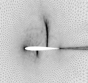
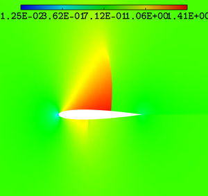
The result that I’m trying to get is something similar to the following picture (my case is 3D):

I’m using the density flow field in order to compute the metric, using mshmet. I haven’t found much documentation about this software, I hope I’m using it correctly.

the command that I use is:
mshmet -temp.mesh -eps 0.0001 -hmin 0.001 -hmax 10
The dentisy flow field is stored in the file .sol with the same name of the mesh. (temp.sol)
Mshmet saves a file temp.new.sol containing the metric. It has 6 columns for each row (vertex).

Then, the new mesh is generate by mmg3d with the followiwng command:
mmg3d_O3 temp.mesh -sol temp.new.sol -hgrad 1.5 -hmin 0.001 -hmax 10

Iterating this procedure, I got this result:

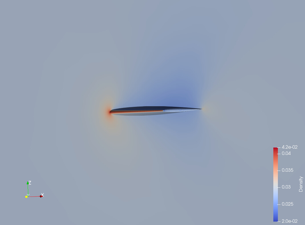
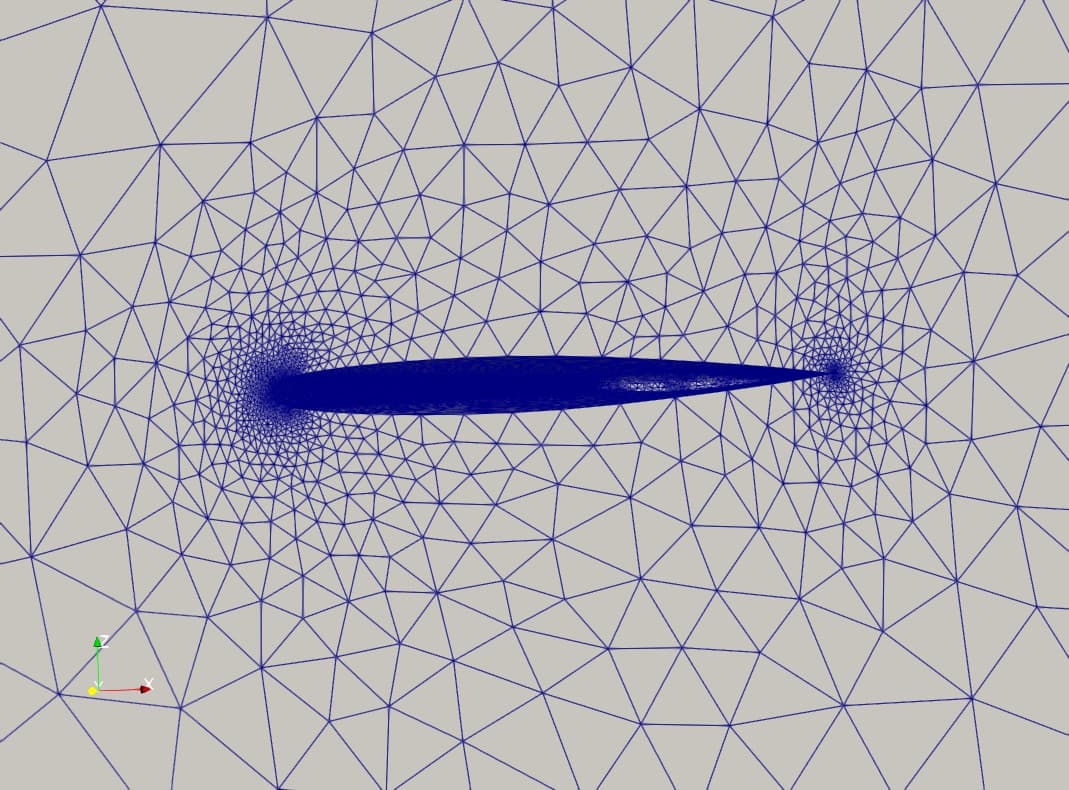
It captures only the density gradient near the stagnation point, but doest not capture the shock.
I’ve already tried varying all the parameters, including the flow field for the computation (I also tryied Mach number), but my result is not close to the expected one.

Can anyone tell me what I’m doing wrong?
I was also wondering the difference between hmin and hmax of mshmet and mmg3d.

[Martin]

Hi @casfra96,

I am a new user of mmg3D and mshmet. I try to do something very similar and I struggle with mshmet as well.

Can you detail how did you store your density field? Which format are you using?

Did you manage to find a solution to your issue?

Thanks,
Martin

[lcirrott]

Hello,
In my experience, mshmet is very sensitive to -eps and -hmin.

This comes from the definition of the metric tensor (see this paper, equation 13). Essentially the metric tensor is defined by taking the eigendecomposition (\lambda_i, \mathbf r_i ) of the Hessian of your solution field, and replacing its eigenvalues to respect minimum and maximum edge sizes:

\mathbf M = \mathbf{ R } \mathbf {\Sigma } \mathbf {R}^T
\sigma_i = \min \left( \max \left( \frac{c | \lambda_i|}{\epsilon}, \frac{1}{h^2_\text{max}} \right), \frac{1}{h^2_\text{min}} \right)

If you take the limit \epsilon \rightarrow 0, you see that the original eigenvalue is imposed as you take smaller and smaller values of -eps. Even with that, if you take h_\text{min} \rightarrow \infty , you see that h_\text{min} is imposed instead of the size coming from your eigenvalue.

My suggestion is to play with the formula knowing that, if you want to impose the sizes coming from variations of your solution field, you want to impose the original eigenvalues as much as possible. Typically this means taking smaller values of -eps as long as smaller values of -hmin to allow smaller sizes in the metric field. The value -hmax is normally more straightforward to adjust.

To answer to the last question: -hmin and -hmax in mshmet are the minimum/maximum edge size you want to be specified in your metric tensor, while these values in mmg are the minimum/maximum edge size you really want in your final mesh (since mmg could slightly modify the metric tensor to account for complex geometrical boundaries).

Hope this helps,

Luca

P.S. Please do not hesitate to visualize the metric file .sol in Medit to see if it has captured the shock, and to share the files so that others can have a try.