
Hello,
Here is a straightforward code (written in Python 3.9 and numpy library) to demonstrate the process of mesh adaptation using mmg executable:
'''
Program to demonstrate the following features of mmg executable:
1. The mesh file format
2. A simple mesh generation using mmg2d
3. The metric file format
4. A simple metric calculation algorithm
5. Multi-stage mesh adaptation process
Note: In a real simulation, all the interactions with mmg will be through
API calls and not using executables.
Useful references & links:
1. https://pages.saclay.inria.fr/frederic.alauzet/proceedings/Frey_Anisotropic%20mesh%20adaptation%20in%203D%20Application%20to%20CFD%20simulations.pdf
2. https://www.mmgtools.org/mmg-remesher-try-mmg/mmg-remesher-tutorials/anisotropic-metric-prescription
3. https://www.mmgtools.org/mmg-remesher-try-mmg/mmg-remesher-tutorials/mmg-remesher-mmg2d/mesh-generation
4. https://theses.hal.science/tel-01284113
Author:
Sourabh Bhat <sourabh.bhat@inria.fr>
'''
import numpy as np
from numpy import sin, arctan
import subprocess
def f(x, y):
# solution function
# change this function as needed
return 0.5 * sin(50*x) + 10 * arctan(0.1 / (sin(5*y) - 2*x))
def hessian_matrix(x, y):
# Note: In a real application, the Hessian needs to be
# computed numerically using solution at the nodes.
# Here, partial derivatives are approximated numerically (of a known function) for convenience.
# replace with analytical functions, if necessary.
dx = 1e-6
dy = 1e-6
d2f_dx2 = (f(x+dx, y) - 2*f(x, y) + f(x-dx, y)) / (dx*dx)
d2f_dy2 = (f(x, y+dy) - 2*f(x, y) + f(x, y-dy)) / (dy*dy)
d2f_dxdy = (f(x+dx, y+dy) - f(x+dx, y-dy) -
f(x-dx, y+dy) + f(x-dx, y-dy)) / (4*dx*dy)
return np.array([[d2f_dx2, d2f_dxdy],
[d2f_dxdy, d2f_dy2]])
# main function
def main():
# Note: In a real simulation, all the interactions with mmg will be through
# api calls and not using executables.
meshfile_path = generate_starting_mesh()
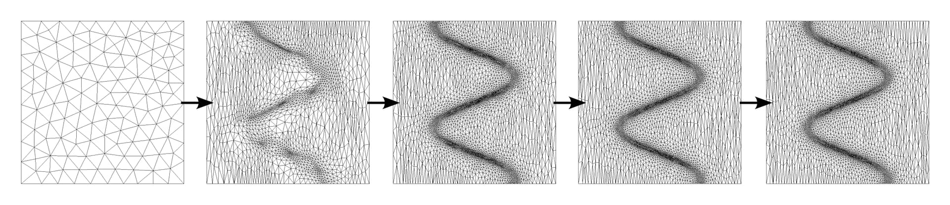
# Note: The following mesh adaptations can be done in a loop :)
# first adaptation
adapt_mesh_using_mmg(meshfile_path)
# second adaptation (with metric computed on adapted mesh)
meshfile_path = meshfile_path.replace(".mesh", ".o.mesh")
adapt_mesh_using_mmg(meshfile_path)
# third adaptation (with metric computed on adapted mesh)
meshfile_path = meshfile_path.replace(".mesh", ".o.mesh")
adapt_mesh_using_mmg(meshfile_path)
# fourth adaptation (with metric computed on adapted mesh)
meshfile_path = meshfile_path.replace(".mesh", ".o.mesh")
adapt_mesh_using_mmg(meshfile_path)
mmg_exe = "mmg2d_O3"
def adapt_mesh_using_mmg(meshfile):
# Steps:
# 1. Write metric to .sol file.
# 2. Call mmg for mesh adaptation.
# Note: In a real application,
# no need to read vertices of current mesh (as they are aready known).
# these are the nodes where current solution and Hessians/metric are available.
# Step 0: read mesh vertices from current mesh
nodes = read_mesh_nodes(meshfile)
# Step 1: compute and write metric to sol file
solution_file = meshfile.replace(".mesh", ".sol")
with open(solution_file, "w") as file:
file.write("MeshVersionFormatted 2" + "\n")
file.write("Dimension 2" + "\n")
file.write("SolAtVertices" + "\n")
file.write(f"{len(nodes)}" + "\n")
file.write(f"1 3" + "\n")
for (x, y) in nodes:
m = metric(x, y)
file.write(f"{m[0,0]} {m[0,1]} {m[1,1]}" + "\n")
file.write("End" + "\n")
# Step 2: Call mmg for mesh adaptation
subprocess.call([mmg_exe,
'-in', meshfile,
'-sol', solution_file])
def metric(x, y):
# A simple definition of metric, for demonstration purposes only!
# In a real appliation, you also need to
# modify the metric based on edge-size constraints, aspect ratio limit, number of elements etc.
hessian = hessian_matrix(x, y)
# make positive definite
evals, evecs = np.linalg.eig(hessian)
abs_evals = np.clip(np.abs(evals), 1e-8, 1e+8)
return evecs * abs_evals @ np.linalg.inv(evecs)
def generate_starting_mesh():
# Note: you can use other software for mesh generation (such as gmsh)
# Here, we are using mmg for mesh generation to keep it simple (and stupid!).
input_geometry = "input.mesh"
vertices = [(-1, -1), (1, -1), (1, 1), (-1, 1)]
edges = [(1, 2), (2, 3), (3, 4), (4, 1)] # edge connectivity
with open(input_geometry, "w") as file:
file.write("MeshVersionFormatted 2" + "\n")
file.write("Dimension 2" + "\n")
file.write("Vertices" + "\n")
file.write(f"{len(vertices)}" + "\n")
for (x, y) in vertices:
file.write(f"{x:10.5f} {y:10.5f} {0:5d}" + "\n")
file.write("Edges" + "\n")
file.write(f"{len(edges)}" + "\n")
# use as per your boundary tags. Here using arbitrary tag number 7
edge_tag = 7
for (start, end) in edges:
file.write(f"{start} {end} {edge_tag}" + "\n")
file.write("End" + "\n")
starting_mesh = "output.mesh"
# call mmg to generate initial mesh
subprocess.call([mmg_exe,
'-hmax', '0.2',
'-in', input_geometry,
'-out', starting_mesh])
return starting_mesh
def read_mesh_nodes(meshfile):
nodes = []
with open(meshfile) as file:
for line in file:
if line.strip() == "Vertices":
break
num_nodes = int(file.readline())
for i in range(num_nodes):
x, y, tag = file.readline().split()
nodes.append((float(x), float(y)))
return nodes
if __name__ == "__main__":
main()
This is a self contained program which generates its own mesh and adapts the mesh using mmg2d. You will need to get mmg from http://www.mmgtools.org/mmg-remesher-downloads or compile it from source to obtain the executable mmg2d_O3. To visualize the generated / adapted mesh you can use Medit (https://github.com/ISCDtoolbox/Medit).
Here is an example function which is used for mesh adaptation:
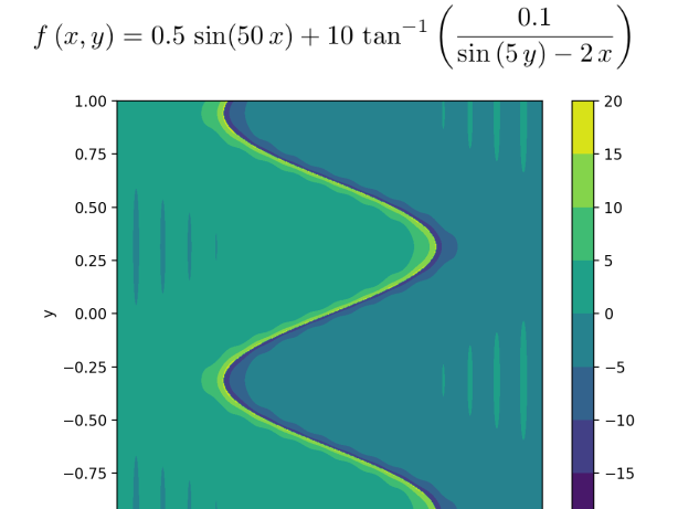
which produces following series of adaptations:
Other references which may be useful:
https://www.mmgtools.org/mmg-remesher-try-mmg/mmg-remesher-tutorials/anisotropic-metric-prescriptionhttps://pages.saclay.inria.fr/frederic.alauzet/proceedings/Frey_Anisotropic%20mesh%20adaptation%20in%203D%20Application%20to%20CFD%20simulations.pdfhttps://www.mmgtools.org/mmg-remesher-try-mmg/mmg-remesher-tutorials/mmg-remesher-mmg2d/mesh-generationhttps://theses.hal.science/tel-01284113
Notes:
- In practical applications, the use of shared library is a preferred way to interact with MMG using API calls. However, this example code will be useful in understanding the algorithm for mesh adaptation.
- In a real application you will have other constraints and requirements for metric calculation, such as element size limits, aspect ratio limits, number of elements etc. Here, a very simple definition of metric is used.
- A few more comments are written in the code at appropriate places.
Cheers!
Sourabh Bhat
CARDAMOM Team, Inria